Algorithms’ complexity analysis - the Big-O Notation
As there usually are multiple ways to solve the given problem, given the multiple algorithms’ implementation, one would find their comparation useful. This is what is algorithm analysis all about. Suppose we want to sum the first n integers: user inputs the number and all integers from 1 till n are summed up. We could do it via iteration like this:
(pseudocode)
1
2
3
4
5
6
7
create function sum(n)
{
 declare integer sum=0
 loop from integer I starting from 1 till n+1
 in every iteration add to sum value of i
 return sum
}
Or using a mathematic shortcut that tells us the sum of first n numbers is one half of product of number n and its larger follower, n+1, like this:
(pseudocode)
1
2
3
4
create function sum(n)
{
return (n*(n+1))/2
}
We don’t need some specialized knowledge in algorithm analyze to figure out that, in terms of simplicity and efficiency, second implementation will have the decisive difference: it will be faster and simpler to calculate the product of two numbers and to half that then to iterate through a list of numbers, adding each one and summing it up in the last iteration. We could easily measure the execution times in any programming language and we would realize the differences. However, it turns out that the execution time is not a good reference for comparing algorithms because it is dependable upon the computer hardware and software configuration. What we need is an algorithm comparison which is not reliant upon the given programming language, style of the coder, machine/operating system internal timer’s configuration, etc. Since we have already defined that the main reference should revolve around algorithm’s executing time, we can deepen the time analysis stating three cases:
- Worst case: defines the input data with which the algorithm runs with the most time (ie. slowest),
- Best case: the fastest algorithm’s run given the input data, and
- Average case: predicts the average time with the random input.
If we are going to exclude the external influences like software and hardware and to focus only on the algorithm’s complexity (which directly influences running time) in relative terms, only our bet is to link inputs with outputs and to see how the output behaves when input changes. Since we can represent any algorithm with a mathematical expression (assuming here it is a function), our aim is to analyze how the execution time changes when we change the input data. If we search for an element in an array of 100 elements applying brute force through iterating all elements and comparing them with the search term (linear search), execution time will surely be shorter opposed to searching 100.000 elements in the same manner. If we take into account two search algorithms and compare their execution time on different input data (array sizes), we can then derive conclusions on how they perform in terms of their best and worst cases.
In this sense, Big-O notation is the upper bound of the given function showing how function (our algorithm) behaves when the argument (input data, variables) tends to enlarge. It is represented as f(x)=O(g(x)), which in computer science translates to function f(x) that approximates given algorithm has an upper bound of output cases in a form of function g(x). That means we defined another function, g(x) which shows the maximum rate of growth for f(x) at larger values of x.
Suppose we represent some algorithm with a function:
1
f(x)=3x^2+30x+300
At the lower values of x, certainly up to 10, the constant 300 is the dominant part of the function, but when the x rises in value it tends to dwarf other parts of the equation, so the part 3x^2 becomes one with the most weight. In fact, we can actually strip the 3 and leave only the x^2 as it contributes by far for most growth. So, we can say that function f(x) has an order of magnitude f(x)=x^2, or say O(x^2). So, in the computer science, Big-O notation shows how the given algorithm will perform in the worst possible case and it can therefore be used to approximate the performance of given algorithm, which then can be compared to other one. There is no automatized way to translate algorithm into meaningful Big-O notation. One needs to analyze the parts of the algorithm counting the steps of the computation and to add their time of execution together. There are some useful guidelines in the process:
- Loops. The execution time of a loop is the execution time of all statements inside a loop multiplied with all iterations. So, execution time = c * x = O(x).
- Nested loops. Multiplication of execution times of all loops, so in case of one outer and one inner loop we have c * x * x = O(x^2).
- Consecutive statements. Sum the execution time of each statement in a code block. For instance:
1
2
3
4
5
6
7
8
9
10
int x=10;
for (int i=0; i<x, i++): // execution x times
{
    Console.WriteLine(i);    // constant time
}
for (int i=0; i<x, i++): // execution x times
{
    for (int j=0; j<x, j++):  // execution x times
        Console.WriteLine ("i value: "+ i+ " and j value: "+ j);
}
which translates to x+c+x^2= O(x^2).
- If statements. Worst execution time translates to the if test itself plus code after if or else statement, whatever is longer to execute. For example:
1
2
3
4
5
6
7
8
if x==0 // constant time
{
  Console.WriteLine("Incorrect");
else
  for (int i=1; i<x; i++) // x times
{
Console.WriteLine("Number is " + i) // constant time
}
so, total time = c+x+c=O(x).
- Logarithmic-complexity statements. If it takes a constant time to reduce the problem size by a fraction, then algorithm is O(logn). For instance:
1
2
3
4
5
6
7
8
9
10
11
void Log(int x)
{
  int i=1;
  while (i<=x)
  {
    i*=2;
    Console.WriteLine(i);
   }
}

Log(100)
Output:
1
2
3
4
5
6
7
2
4
8
16
32
64
128
The loop exits after n times so we can define 2^k=x => k=logn (base 2 rather than 10). So, total time here is O(logn).
Generally, we can establish the estimates for the commonly used mathematical expressions as follows:
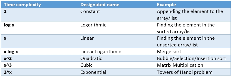 Figure 1: Common time complexities
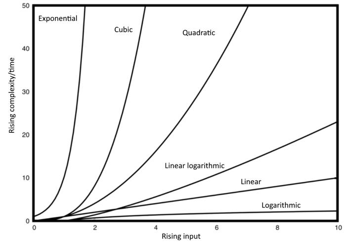 Figure 2: Graphical representation of some time complexities
One can dive more into mathematics and complexity theory to further study the best and average cases as well as amortized analysis; however, for most approximations and comparations the worst-case algorithm’s behavior depicted by the Big-O notation suffices.
Interpretation of the Big-O notation’s outcome is also worth discussing. One has to bear in mind constantly that the calculated O(g(x)) is the upper bond of the notation, meaning the worst-possible case. If one algorithm gives O(x) and another O(x^2), that does not mean the first one is faster; rather that the second one will tend to have worse outcome on the large enough input. So, the comparative analysis via Big-O notation will have some drawbacks if one wants to find best running time for given algorithm, and then the analysis must be broadened by introducing another notation, Omega-notation, which we will leave for another time.
Conclusion
In this article we have shown that we can design self-made tests in our particular programming language to measure the executional timing of our code, however this does have some serious drawbacks as the results are not comparable but rather very dependable upon a number of circumstances. Complexity theory gives us the approximative tools to translate an algorithm into set of mathematical statements and to estimate its complexity giving estimates on each part of the code. Such results can be then compared to other algorithms’ estimates within given mathematical boundaries. This analysis using Big-O notation can give a reasonably detailed picture on the worst-possible case of algorithm’s complexity.